Chapter 7 Bayesian Models 1.2 LACs

The real question: why do we repeat the process on liberal arts colleges again?

Answer: Liberal arts colleges fall under an entirely separate ranking list and often have different characteristics (e.g. size and location, private vs public). We repeat the process to observe the similarity and differences between universities and liberal arts colleges.

7.1 Model 0

Ranking by one year of SAT score: with intuition from \(\text{hist}(\sqrt{1/rgamma(10000,a,b)})\).

7.1.1 First Impression

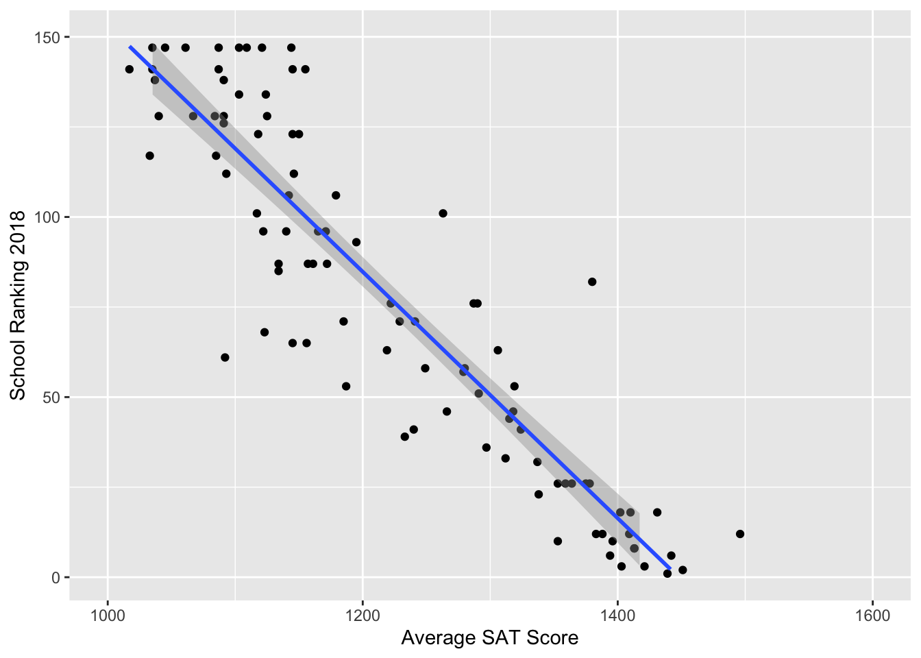
Since it appears to be a linear relationship, we again proceeded with a linear model.

7.1.2 Building the model

Let \(Y_i\) denote the predicted ranking of a liberal arts college in Year 2018. \(Y_i\) is predicted by

\[X_i = \text{student mean SAT score of Year 2016-17}\]

Our model can be written as:

\[\begin{align} Y_i & \sim N(\beta_0 + \beta_1X_i,\tau_0) \\ \beta_0 & \sim N(300,250000^{-1}) \\ \beta_1 & \sim N(0,100^{-1}) \\ \tau_0 & \sim Gamma(7,4000) \end{align}\]

# DEFINE the model
liberal_model_0 <- "model{
    for(i in 1:length(y)) {
        # Data model
        y[i] ~ dnorm(beta0 + beta1 * x[i], tau0)
    }

    # Priors for theta
    beta0 ~ dnorm(300,1/250000)
    beta1 ~ dnorm(0, 1/100)
    tau0 ~ dgamma(7,4000)

}"


# COMPILE the model
model_data4 <- data.frame(y = full_LiberalArts$Y2018, x = full_LiberalArts$SAT_AVG_1617)
model_data4 <- na.omit(model_data4)

liberal_jags_0 <- jags.model(textConnection(liberal_model_0), 
    data = list(y = model_data4$y, x = model_data4$x),
    inits = list(.RNG.name = "base::Wichmann-Hill", .RNG.seed = 454))

## Compiling model graph
##    Resolving undeclared variables
##    Allocating nodes
## Graph information:
##    Observed stochastic nodes: 101
##    Unobserved stochastic nodes: 3
##    Total graph size: 396
## 
## Initializing model

# SIMULATE the model
liberal_sim_0 <- coda.samples(liberal_jags_0,
    variable.names = c("beta0", "beta1", "tau0"),
    n.iter = 10000)

# STORE the chains in a data frame
liberal_chains_0 <- data.frame(liberal_sim_0[[1]])

7.1.3 Model summary

summary(liberal_sim_0)

## 
## Iterations = 1:10000
## Thinning interval = 1 
## Number of chains = 1 
## Sample size per chain = 10000 
## 
## 1. Empirical mean and standard deviation for each variable,
##    plus standard error of the mean:
## 
##            Mean        SD  Naive SE Time-series SE
## beta0 -0.614922 1.583e+01 1.583e-01      2.144e+00
## beta1  0.021724 1.296e-02 1.296e-04      1.767e-03
## tau0   0.003849 5.113e-04 5.113e-06      5.914e-06
## 
## 2. Quantiles for each variable:
## 
##             2.5%        25%       50%       75%     97.5%
## beta0 -31.655750 -11.608615 -1.094746 10.751901 29.460108
## beta1  -0.003149   0.012368  0.022064  0.030707  0.047298
## tau0    0.002903   0.003495  0.003829  0.004177  0.004907

7.1.4 Posterior inference

For an unknown liberal arts college with a mean student SAT score of 1450 (e.g. Bvictor College), we could predict its ranking from our rjags simulation.

liberal_chains_0 <- liberal_chains_0 %>%
  mutate(ranking_new = rnorm(10000, mean = beta0 + beta1*1450, sd = (1/tau0)^(1/2)))

liberal_chains_0 %>%
  summarize(quantile(ranking_new,0.025),quantile(ranking_new,0.975))

##   quantile(ranking_new, 0.025) quantile(ranking_new, 0.975)
## 1                    -1.300984                     63.18926

A \(95\%\) credible interval is \((-1,63)\). Due to restrictions of this one-predictor model, we expect to see an improvement in later models.

7.2 Model 1

Ranking by three years of SAT score. This is the best Bayesian model one can ever come up with.

Just Kidding.

As we discussed earlier in Chapter 6, Model 1 is overwhelmingly multicollinear; Model 1 is a sufficient sustitute if we want to look at the relationship between ranking and SAT score.

7.3 Model 2

2018 U.S. News Ranking by average SAT score and admissions rate of Year 2017.

7.3.1 First Impression

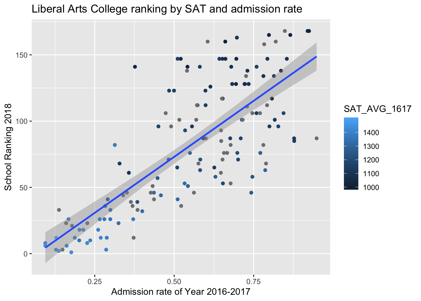
There’s a strong positive relationship between the admission rate of colleges and college ranking (a larger number in college ranking is worse). From color gradient of points, we can see that schools with higher SAT averages tend to be better ranked.

7.3.2 Building the model

7.3.2.1 Step 1

A linear model provides some intuition about how the priors might be constructed.

summary(lm(full_LiberalArts$Y2018 ~ full_LiberalArts$SAT_AVG_1617 + full_LiberalArts$ADM_RATE_1617))

## 
## Call:
## lm(formula = full_LiberalArts$Y2018 ~ full_LiberalArts$SAT_AVG_1617 + 
##     full_LiberalArts$ADM_RATE_1617)
## 
## Residuals:
##     Min      1Q  Median      3Q     Max 
## -50.679  -9.613  -0.042  10.169  59.538 
## 
## Coefficients:
##                                 Estimate Std. Error t value Pr(>|t|)    
## (Intercept)                    430.23894   34.40379  12.506   <2e-16 ***
## full_LiberalArts$SAT_AVG_1617   -0.30402    0.02336 -13.012   <2e-16 ***
## full_LiberalArts$ADM_RATE_1617  37.57722   13.59032   2.765   0.0068 ** 
## ---
## Signif. codes:  0 '***' 0.001 '**' 0.01 '*' 0.05 '.' 0.1 ' ' 1
## 
## Residual standard error: 19.48 on 98 degrees of freedom
##   (48 observations deleted due to missingness)
## Multiple R-squared:  0.8577, Adjusted R-squared:  0.8548 
## F-statistic: 295.3 on 2 and 98 DF,  p-value: < 2.2e-16

7.3.2.2 Step 2

Next, we construct a hierarchical model of

\[Y_i = \text{the predicted 2018 ranking of a liberal arts college}\]

\[\begin{align} X_{1i} & = \text{student mean SAT score of Year 2016-17} \\ X_{2i} & = \text{admissions rate during Year 2016-17} \end{align}\]

where

\[\begin{align} Y_i & \sim N(\beta_{0i} + \beta_{1i}X_{1i} + \beta_{2i}X_{2i}, \tau_{\text{big}[i]}) \\ \beta_{0i} & \sim N(b_0,\tau_0) \\ \beta_{1i} & \sim N(b_1,\tau_1) \\ \beta_{2i} & \sim N(b_2,\tau_2) \\ \tau_{\text{big}[i]} & \sim Gamma(s,r) \\ b_0 & \sim N(180,4000^{-1}) \\ \tau_0 & \sim N(30, 1/9) \\ b_1 & \sim N(-0.1,0.001^{-1}) \\ \tau_1 & \sim N(1000, 0.001^{-1}) \\ b_2 & \sim N(80,100^{-1}) \\ \tau_2 & \sim N(10, 1) \\ s & \sim N(7,1) \\ r & \sim N(10000, 10000^{-1}) \end{align}\]

liberal_model_2 <- "model{  
    # Data: observations
    for(i in 1:length(y)) {
        y[i] ~ dnorm(beta0[i] + beta1[i]*x1[i] + beta2[i]*x2[i], tau_big[i])

        # Data: subjects
        beta0[i] ~ dnorm(b0, tau0)
        beta1[i] ~ dnorm(b1,tau1)
        beta2[i] ~ dnorm(b2,tau2)
        tau_big[i] ~ dgamma(s,r)
    }

    # Hyperpriors
    b0 ~ dnorm(180,1/4000)
    tau0 ~ dnorm(30, 1/9)
    b1 ~ dnorm(-0.1,1000)
    tau1 ~ dnorm(1000,1000) 
    b2 ~ dnorm(80,1/100)
    tau2 ~ dnorm(10,1)
    s ~ dnorm(7,1)
    r ~ dnorm(10000, 1/10000)
}"

# COMPILE

y <- full_LiberalArts$Y2018

model_data5 <- as.data.frame(cbind(y, x1 = full_LiberalArts$SAT_AVG_1617, x2 = full_LiberalArts$ADM_RATE_1617))
model_data5 <- na.omit(model_data5)

liberal_jags_2 <- jags.model(textConnection(liberal_model_2), 
    data = list(y = model_data5$y, x1 = model_data5$x1, x2 = model_data5$x2),
    inits=list(.RNG.name = "base::Wichmann-Hill", .RNG.seed = 454))

## Compiling model graph
##    Resolving undeclared variables
##    Allocating nodes
## Graph information:
##    Observed stochastic nodes: 101
##    Unobserved stochastic nodes: 412
##    Total graph size: 1035
## 
## Initializing model

# SIMULATE the model
liberal_sim_2 <- coda.samples(liberal_jags_2,
    variable.names = c("b0","tau0","b1","tau1","b2","tau2","s","r"),
    n.iter = 10000)

# STORE the chains in a data frame
liberal_chains_2 <- data.frame(liberal_sim_2[[1]])

7.3.3 Model summary

summary(liberal_sim_2)

## 
## Iterations = 1001:11000
## Thinning interval = 1 
## Number of chains = 1 
## Sample size per chain = 10000 
## 
## 1. Empirical mean and standard deviation for each variable,
##    plus standard error of the mean:
## 
##            Mean       SD  Naive SE Time-series SE
## b0     178.4834  0.56301 0.0056301      0.1895714
## b1      -0.1090  0.02947 0.0002947      0.0039424
## b2      43.1793  5.95589 0.0595589      4.0299101
## r    10016.5430 99.18842 0.9918842      1.2203209
## s        0.1517  0.01632 0.0001632      0.0009056
## tau0    30.1001  3.00404 0.0300404      0.0510047
## tau1   999.9994  0.03244 0.0003244      0.0004133
## tau2    10.0017  1.01154 0.0101154      0.0176700
## 
## 2. Quantiles for each variable:
## 
##           2.5%       25%        50%        75%      97.5%
## b0    177.2556  178.0642   178.5477  1.789e+02  1.793e+02
## b1     -0.1706   -0.1287    -0.1086 -8.759e-02 -5.609e-02
## b2     33.4737   38.3188    42.4722  4.779e+01  5.528e+01
## r    9819.6765 9950.7472 10016.6172  1.008e+04  1.022e+04
## s       0.1220    0.1402     0.1511  1.627e-01  1.850e-01
## tau0   24.2727   28.0611    30.0777  3.214e+01  3.610e+01
## tau1  999.9360  999.9776   999.9993  1.000e+03  1.000e+03
## tau2    8.0292    9.3206     9.9837  1.067e+01  1.202e+01

7.3.4 Posterior inference

For an unknown Liberal Arts College with student mean SAT score of 1450 and an admission rate of \(30\%\) (e.g. Dvictor college), we could predict its ranking from our rjags simulation.

liberal_chains_2 <- liberal_chains_2 %>%
  mutate(beta0_new = rnorm(10000,b0,(1/tau0)^(1/2))) %>%
           mutate(beta1_new = rnorm(10000,b1,(1/tau1)^(1/2))) %>%
           mutate(beta2_new = rnorm(10000,b2,(1/tau2)^(1/2))) %>%
           mutate(tau_big_new = rgamma(10000,s,r)) %>%
           mutate(ranking_new = rnorm(10000, mean = beta0_new + beta1_new * 1450 + beta2_new * 0.3, sd = (1/tau_big_new)^(1/2)))

liberal_chains_2 %>%
  summarize(quantile(ranking_new,0.025),quantile(ranking_new,0.975))

##   quantile(ranking_new, 0.025) quantile(ranking_new, 0.975)
## 1                     -2231220                      2227442

A \(95\%\) credible interval is not pretty! This means that we over-evaluate the variability of a lot of predictors.

7.4 Future steps

Given the problem that we encounter at Dvictor College, we also need to pay attention to narrowing the variability in our Bayesian models. (which really teaches us a lesson: simple is good; a complicated hierarchical model is not always helpful!)