Chapter 6 Bayesian Models 1.1 Universities

How will we simulate what we want to know?

HINT: Start SIMPLE

6.1 Model 0

Ranking by one year of SAT score: with intuition from \(\text{hist}(\sqrt{1/rgamma(10000,a,b)})\).

6.1.1 First Impression

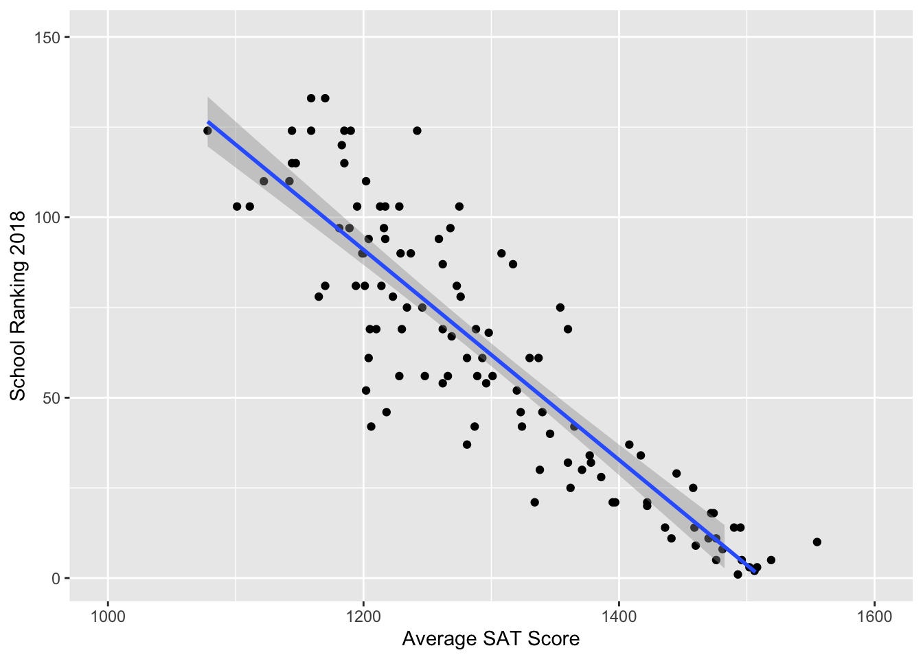
It appears to be a linear relationship! So, we proceeded to create a normal prior made of a linear combination of values.

6.1.2 Building the model

Let \(Y_i\) denote the predicted ranking of a university in Year 2018. \(Y_i\) is predicted by

\[X_i = \text{student mean SAT score of Year 2016-17}\]

Our model can be written as:

\[\begin{align} Y_i & \sim N(\beta_0 + \beta_1X_i,\tau_0) \\ \beta_0 & \sim N(300,250000^{-1}) \\ \beta_1 & \sim N(0,100^{-1}) \\ \tau_0 & \sim Gamma(7,4000) \end{align}\]

# DEFINE the model
university_model_0 <- "model{
    for(i in 1:length(y)) {
        # Data model
        y[i] ~ dnorm(beta0 + beta1 * x[i], tau0)
    }

    # Priors for theta
    beta0 ~ dnorm(300,1/250000)
    beta1 ~ dnorm(0, 1/100)
    tau0 ~ dgamma(7,4000)

}"


# COMPILE the model
model_data0 <- data.frame(y = fullUniversity$Y2018, x = fullUniversity$SAT_AVG_1617)
model_data0 <- na.omit(model_data0)

university_jags_0 <- jags.model(textConnection(university_model_0), 
    data = list(y = model_data0$y, x = model_data0$x),
    inits = list(.RNG.name = "base::Wichmann-Hill", .RNG.seed = 454))

## Compiling model graph
##    Resolving undeclared variables
##    Allocating nodes
## Graph information:
##    Observed stochastic nodes: 114
##    Unobserved stochastic nodes: 3
##    Total graph size: 440
## 
## Initializing model

# SIMULATE the model
university_sim_0 <- coda.samples(university_jags_0,
    variable.names = c("beta0", "beta1", "tau0"),
    n.iter = 10000)

# STORE the chains in a data frame
university_chains_0 <- data.frame(university_sim_0[[1]])

6.1.3 Model summary

summary(university_sim_0)

## 
## Iterations = 1:10000
## Thinning interval = 1 
## Number of chains = 1 
## Sample size per chain = 10000 
## 
## 1. Empirical mean and standard deviation for each variable,
##    plus standard error of the mean:
## 
##             Mean        SD  Naive SE Time-series SE
## beta0 403.411563 3.227e+01 3.227e-01      4.714e+00
## beta1  -0.263423 2.472e-02 2.472e-04      3.617e-03
## tau0    0.002421 3.279e-04 3.279e-06      1.303e-05
## 
## 2. Quantiles for each variable:
## 
##            2.5%        25%        50%        75%      97.5%
## beta0 355.59133 390.793008 405.743679 421.198553 447.191343
## beta1  -0.29699  -0.277127  -0.265219  -0.253713  -0.226779
## tau0    0.00182   0.002212   0.002415   0.002628   0.003062

6.1.4 Posterior inference

For an unknown university with a mean student SAT score of 1450 (e.g. Bvictor University), we could predict its ranking from our rjags simulation.

university_chains_0 <- university_chains_0 %>%
  mutate(ranking_new = rnorm(10000, mean = beta0 + beta1*1450, sd = (1/tau0)^(1/2)))

university_chains_0 %>%
  summarize(quantile(ranking_new,0.025),quantile(ranking_new,0.975))

##   quantile(ranking_new, 0.025) quantile(ranking_new, 0.975)
## 1                    -18.35693                     62.67805

A \(95\%\) credible interval is \((-20,62)\).Unfortunately, we ended up with range that included negative values, which led us to believe that we either needed more predictors, or we needed to change the model type. Due to restrictions of this one-predictor model, we expect to see an improvement in later models. We decided to try adding more predictors first.

6.2 Model 1

6.2.1 First Impression

It’s harder to make predictions (and as it turns out, hard to make visualizations as well) with three years’ SAT score in the same linear model, as we can foresee significant multicollinearity. This is clearly seen that the coefficient for SAT average of Year 2014-15 (SAT_AVG_1415) variable is positive, meaning that school ranking worsens as the average SAT score increases.

To further test our thinking, we created a linear model university_linear_1. From the ANOVA summary, we see that any one of these variables should be sufficient.

university_linear_1 <- lm(as.numeric(Y2018) ~ SAT_AVG_1617 + SAT_AVG_1516 + SAT_AVG_1415, fullUniversity)

summary(university_linear_1)

## 
## Call:
## lm(formula = as.numeric(Y2018) ~ SAT_AVG_1617 + SAT_AVG_1516 + 
##     SAT_AVG_1415, data = fullUniversity)
## 
## Residuals:
##      Min       1Q   Median       3Q      Max 
## -104.127   -8.988   -2.062   12.129   38.789 
## 
## Coefficients:
##               Estimate Std. Error t value Pr(>|t|)    
## (Intercept)  415.49873   20.70087  20.072   <2e-16 ***
## SAT_AVG_1617  -0.04769    0.14485  -0.329    0.743    
## SAT_AVG_1516  -0.26890    0.18977  -1.417    0.159    
## SAT_AVG_1415   0.04301    0.16163   0.266    0.791    
## ---
## Signif. codes:  0 '***' 0.001 '**' 0.01 '*' 0.05 '.' 0.1 ' ' 1
## 
## Residual standard error: 19.68 on 110 degrees of freedom
##   (6 observations deleted due to missingness)
## Multiple R-squared:  0.7292, Adjusted R-squared:  0.7218 
## F-statistic: 98.75 on 3 and 110 DF,  p-value: < 2.2e-16

anova(university_linear_1)

## Analysis of Variance Table
## 
## Response: as.numeric(Y2018)
##               Df Sum Sq Mean Sq  F value Pr(>F)    
## SAT_AVG_1617   1 113627  113627 293.4484 <2e-16 ***
## SAT_AVG_1516   1   1052    1052   2.7173 0.1021    
## SAT_AVG_1415   1     27      27   0.0708 0.7907    
## Residuals    110  42594     387                    
## ---
## Signif. codes:  0 '***' 0.001 '**' 0.01 '*' 0.05 '.' 0.1 ' ' 1

We decided to model ranking by using the three years of average SAT scores. Through summary analysis and an analysis of variance (ANOVA), the three predictors are multicollinear, meaning that this may not be a significantly better model than Model 0.

For the sake of scientific experiment (and to catch the audience’s interest), we still did a Bayesian model and Bayesian posterior inference. We found out that this model does a slightly better job at predicting college rankings (by eliminating negative rankings) because it naturally contains more information as we increase the number of predictors. The change is not significant enough to call it an improvement.

6.2.2 Building the model

Similarly, we construct a linear regression model of

\[Y_i = \text{the predicted 2018 ranking of a university}\] by

\[\begin{align} X_{1i} & = \text{student mean SAT score of Year 2014-15} \\ X_{2i} & = \text{student mean SAT score of Year 2015-16} \\ X_{3i} & = \text{student mean SAT score of Year 2016-17} \end{align}\]

where

\[\begin{align} Y_i & \sim N(\beta_0 + \beta_1X_{1i} + \beta_2X_{2i} + \beta_3X_{3i},\tau_{\text{big}}) \\ \beta_0 & \sim N(0,250000^{-1}) \\ \beta_1 & \sim N(0,0.01^{-1}) \\ \beta_2 & \sim N(0,0.01^{-1}) \\ \beta_3 & \sim N(0,0.01^{-1}) \\ \tau_{\text{big}} & \sim Gamma(7,1000) \end{align}\]

university_model_1 <- "model{  
    # Data: observations
    for(i in 1:length(y)) {
        y[i] ~ dnorm(beta0 + beta1*x1[i] + beta2*x2[i] + beta3*x3[i], tau_big)
    }

        # Data: subjects
        beta0 ~ dnorm(0,1/250000)
        beta1 ~ dnorm(0,100)
        beta2 ~ dnorm(0,100)
        beta3 ~ dnorm(0,100)
        tau_big ~ dgamma(7,1000)

}"

# COMPILE

y <- fullUniversity$Y2018

model_data1 <- as.data.frame(cbind(y, x1 = fullUniversity$SAT_AVG_1415, x2 = fullUniversity$SAT_AVG_1516, x3 = fullUniversity$SAT_AVG_1617))
model_data1 <- na.omit(model_data1)

university_jags_1 <- jags.model(textConnection(university_model_1), 
    data = list(y = model_data1$y, x1 = model_data1$x1, x2 = model_data1$x2, x3 = model_data1$x3),
    inits=list(.RNG.name = "base::Wichmann-Hill", .RNG.seed = 454))

## Compiling model graph
##    Resolving undeclared variables
##    Allocating nodes
## Graph information:
##    Observed stochastic nodes: 114
##    Unobserved stochastic nodes: 5
##    Total graph size: 876
## 
## Initializing model

# SIMULATE the model
university_sim_1 <- coda.samples(university_jags_1,
    variable.names = c("beta0","beta1","beta2","beta3","tau_big"),
    n.iter = 10000)

# STORE the chains in a data frame
university_chains_1 <- data.frame(university_sim_1[[1]])

6.2.3 Model summary

summary(university_sim_1)

## 
## Iterations = 1:10000
## Thinning interval = 1 
## Number of chains = 1 
## Sample size per chain = 10000 
## 
## 1. Empirical mean and standard deviation for each variable,
##    plus standard error of the mean:
## 
##               Mean        SD  Naive SE Time-series SE
## beta0   409.864989 3.553e+01 3.553e-01      5.783e+00
## beta1     0.001373 1.078e-01 1.078e-03      1.120e-01
## beta2    -0.179656 7.938e-02 7.938e-04      4.684e-02
## beta3    -0.090932 7.417e-02 7.417e-04      5.086e-02
## tau_big   0.002781 4.008e-04 4.008e-06      2.714e-05
## 
## 2. Quantiles for each variable:
## 
##               2.5%        25%        50%        75%      97.5%
## beta0   345.977738 400.686962 414.807439 427.055384 447.427911
## beta1    -0.224077  -0.074142   0.033869   0.084271   0.127709
## beta2    -0.304552  -0.247353  -0.181364  -0.127231  -0.006660
## beta3    -0.212426  -0.151206  -0.106569  -0.025275   0.034454
## tau_big   0.002051   0.002538   0.002778   0.003029   0.003556

6.2.4 Posterior inference

For an unknown university with three years’ mean student SAT score of 1450, 1440, 1420 (e.g. Cvictor University), we could predict its ranking from our rjags simulation.

university_chains_1 <- university_chains_1 %>%
  mutate(ranking_new = rnorm(10000, mean = beta0 + beta1*1450 + beta2*1440 +beta3*1420, sd = (1/tau_big)^(1/2)))

university_chains_1 %>%
  summarize(quantile(ranking_new,0.025),quantile(ranking_new,0.975))

##   quantile(ranking_new, 0.025) quantile(ranking_new, 0.975)
## 1                    -13.99412                     62.48092

A \(95\%\) credible interval is \((-14,64)\). The \(95\%\) credible interval in the new model does a better job at eliminating negative rankings, which are impossible in reality.

6.3 Model 2

2018 U.S. News Ranking by average SAT score and admissions rate of Year 2017.

6.3.1 First Impression

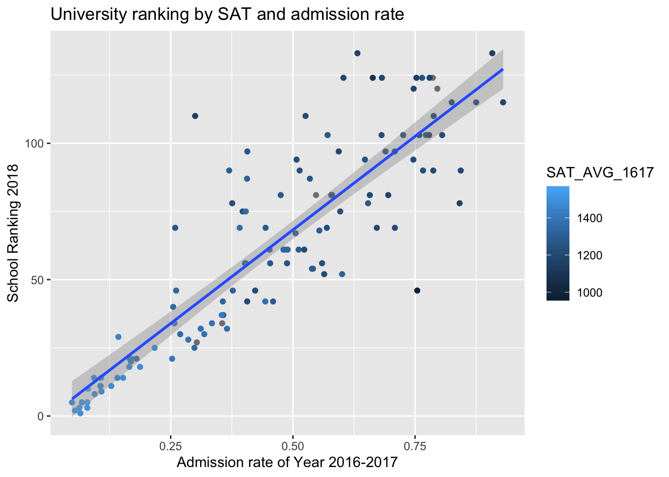
There’s a strong positive relationship between the admission rate of colleges and college ranking (a larger number in college ranking is worse). From color gradient of points, we can see that schools with higher SAT averages tend to be better ranked.

6.3.2 Building the model

6.3.2.1 Step 1

A linear model provides some intuition about how the priors might be constructed.

summary(lm(fullUniversity$Y2018 ~ fullUniversity$SAT_AVG_1617 + fullUniversity$ADM_RATE_1617))

## 
## Call:
## lm(formula = fullUniversity$Y2018 ~ fullUniversity$SAT_AVG_1617 + 
##     fullUniversity$ADM_RATE_1617)
## 
## Residuals:
##     Min      1Q  Median      3Q     Max 
## -78.978  -9.142  -1.986   8.865  43.380 
## 
## Coefficients:
##                              Estimate Std. Error t value Pr(>|t|)    
## (Intercept)                  172.5262    45.1297   3.823 0.000218 ***
## fullUniversity$SAT_AVG_1617   -0.1150     0.0301  -3.822 0.000219 ***
## fullUniversity$ADM_RATE_1617  84.8854    14.8094   5.732 8.66e-08 ***
## ---
## Signif. codes:  0 '***' 0.001 '**' 0.01 '*' 0.05 '.' 0.1 ' ' 1
## 
## Residual standard error: 17.42 on 111 degrees of freedom
##   (6 observations deleted due to missingness)
## Multiple R-squared:  0.7858, Adjusted R-squared:  0.7819 
## F-statistic: 203.6 on 2 and 111 DF,  p-value: < 2.2e-16

6.3.2.2 Step 2

Next, we construct a hierarchical model (because we just learned this and wanted to show off) of

\[Y_i = \text{the predicted 2018 ranking of a university}\] by

\[\begin{align} X_{1i} & = \text{student mean SAT score of Year 2016-17} \\ X_{2i} & = \text{admissions rate during Year 2016-17} \end{align}\]

where

\[\begin{align} Y_i & \sim N(\beta_{0i} + \beta_{1i}X_{1i} + \beta_{2i}X_{2i}, \tau_{\text{big},i}) \\ \beta_{0i} & \sim N(b_0,\tau_0) \\ \beta_{1i} & \sim N(b_1,\tau_1) \\ \beta_{2i} & \sim N(b_2,\tau_2) \\ \tau_{\text{big},i} & \sim Gamma(s,r) \\ b_0 & \sim N(180,4000^{-1}) \\ \tau_0 & \sim N(30, 1/9) \\ b_1 & \sim N(-0.1,0.001^{-1}) \\ \tau_1 & \sim N(1000, 0.001^{-1}) \\ b_2 & \sim N(80,100^{-1}) \\ \tau_2 & \sim N(10, 1) \\ s & \sim N(7,1) \\ r & \sim N(10000, 10000^{-1}) \end{align}\]

university_model_2 <- "model{  
    # Data: observations
    for(i in 1:length(y)) {
        y[i] ~ dnorm(beta0[i] + beta1[i]*x1[i] + beta2[i]*x2[i], tau_big[i])

        # Data: subjects
        beta0[i] ~ dnorm(b0, tau0)
        beta1[i] ~ dnorm(b1,tau1)
        beta2[i] ~ dnorm(b2,tau2)
        tau_big[i] ~ dgamma(s,r)
    }

    # Hyperpriors
    b0 ~ dnorm(180,1/4000)
    tau0 ~ dnorm(30, 1/9)
    b1 ~ dnorm(-0.1,1000)
    tau1 ~ dnorm(1000,1000) 
    b2 ~ dnorm(80,1/100)
    tau2 ~ dnorm(10,1)
    s ~ dnorm(7,1)
    r ~ dnorm(10000, 1/10000)
}"

# COMPILE

y <- fullUniversity$Y2018

model_data2 <- as.data.frame(cbind(y, x1 = fullUniversity$SAT_AVG_1617, x2 = fullUniversity$ADM_RATE_1617))
model_data2 <- na.omit(model_data2)

university_jags_2 <- jags.model(textConnection(university_model_2), 
    data = list(y = model_data2$y, x1 = model_data2$x1, x2 = model_data2$x2),
    inits=list(.RNG.name = "base::Wichmann-Hill", .RNG.seed = 454))

## Compiling model graph
##    Resolving undeclared variables
##    Allocating nodes
## Graph information:
##    Observed stochastic nodes: 114
##    Unobserved stochastic nodes: 464
##    Total graph size: 1165
## 
## Initializing model

# SIMULATE the model
university_sim_2 <- coda.samples(university_jags_2,
    variable.names = c("b0","tau0","b1","tau1","b2","tau2","s","r"),
    n.iter = 10000)

# STORE the chains in a data frame
university_chains_2 <- data.frame(university_sim_2[[1]])

6.3.3 Model summary

summary(university_sim_2)

## 
## Iterations = 1001:11000
## Thinning interval = 1 
## Number of chains = 1 
## Sample size per chain = 10000 
## 
## 1. Empirical mean and standard deviation for each variable,
##    plus standard error of the mean:
## 
##          Mean        SD  Naive SE Time-series SE
## b0    181.003  0.866642 8.666e-03      0.4845152
## b1     -0.122  0.003986 3.986e-05      0.0001962
## b2     86.978  2.748797 2.749e-02      2.0167560
## r    9978.437 98.495695 9.850e-01      1.3555384
## s       9.367  0.854744 8.547e-03      0.0428560
## tau0   29.903  3.051727 3.052e-02      0.0544687
## tau1 1000.000  0.031393 3.139e-04      0.0003934
## tau2   10.021  1.000127 1.000e-02      0.0179231
## 
## 2. Quantiles for each variable:
## 
##           2.5%       25%      50%        75%      97.5%
## b0    179.2258  180.2942  181.163   181.6543   182.5227
## b1     -0.1298   -0.1247   -0.122    -0.1193    -0.1143
## b2     80.6675   85.0648   87.714    89.2203    90.5414
## r    9784.6197 9912.1376 9978.523 10044.9089 10170.4126
## s       7.7114    8.7880    9.345     9.9331    11.0906
## tau0   23.8816   27.8340   29.879    31.9392    35.9038
## tau1  999.9366  999.9792 1000.000  1000.0208  1000.0615
## tau2    8.0599    9.3477   10.030    10.6819    12.0006

6.3.4 Posterior inference

For an unknown university with student mean SAT score of 1450 and an admission rate of \(30\%\) (e.g. Dvictor University), we could predict its ranking from our rjags simulation.

university_chains_2 <- university_chains_2 %>%
  mutate(beta0_new = rnorm(10000,b0,(1/tau0)^(1/2))) %>%
           mutate(beta1_new = rnorm(10000,b1,(1/tau1)^(1/2))) %>%
           mutate(beta2_new = rnorm(10000,b2,(1/tau2)^(1/2))) %>%
           mutate(tau_big_new = rgamma(10000,s,r)) %>%
           mutate(ranking_new = rnorm(10000, mean = beta0_new + beta1_new * 1450 + beta2_new * 0.3, sd = (1/tau_big_new)^(1/2)))

university_chains_2 %>%
  summarize(quantile(ranking_new,0.025),quantile(ranking_new,0.975))

##   quantile(ranking_new, 0.025) quantile(ranking_new, 0.975)
## 1                    -87.00093                     142.8536

A \(95\%\) credible interval is \((-86,142)\). The \(95\%\) credible interval does a poor job at eliminating negative rankings or making an accurate prediction. We propose that this may be due to the variability of the priors and hyperpriors set in our Hierarchical Model.

6.4 Future steps

Next, we plan to incorporate more predictive variables of ranking \(y_i\). Since some predictors we choose are correlated, we will also emphasize on reflecting that in our models.