4.3 Following up on Bernoulli

Suppose $X$ is binomially distributed:

$$X\sim Bin(n,\theta) \\ f(x|\theta) = {n\choose x} \theta^x (1-\theta)^{n-x}$$

From the warmup, given that $E(X)=p$, we know that

$$\begin{aligned} I(\theta) & = -E_{\theta} \left[ \frac{d^2 log f(x|\theta)}{d\theta^2}\right] \\ & = \frac{1}{\theta (1-\theta)} \end{aligned}$$

Then $\pi_J(\theta) = I(\theta)^{\frac{1}{2}} \propto \theta^{\frac{1}{2}}(1-\theta)^{\frac{1}{2}}$, so the Jeffreys prior has the distribution of a $Beta\left(\frac{1}{2},\frac{1}{2}\right)$ density. Below, we can see the distributions of a $Beta\left(\frac{1}{2},\frac{1}{2}\right)$ and a $Beta(1, 1)$, or flat prior.

library(ggplot2)
library(reshape2)

x <- seq(0,1,length=200)
beta_dist <- data.frame(cbind(x, dbeta(x,1,1), dbeta(x,0.5,0.5)))

colnames(beta_dist) <- c("x","a=1 b=1","a=0.5 b=0.5")

beta_dist <- melt(beta_dist,x)

g <- ggplot(beta_dist, aes(x,value, color=variable))
g+geom_line() + labs(title="Beta Distribution") + labs(x="Probability", y="density")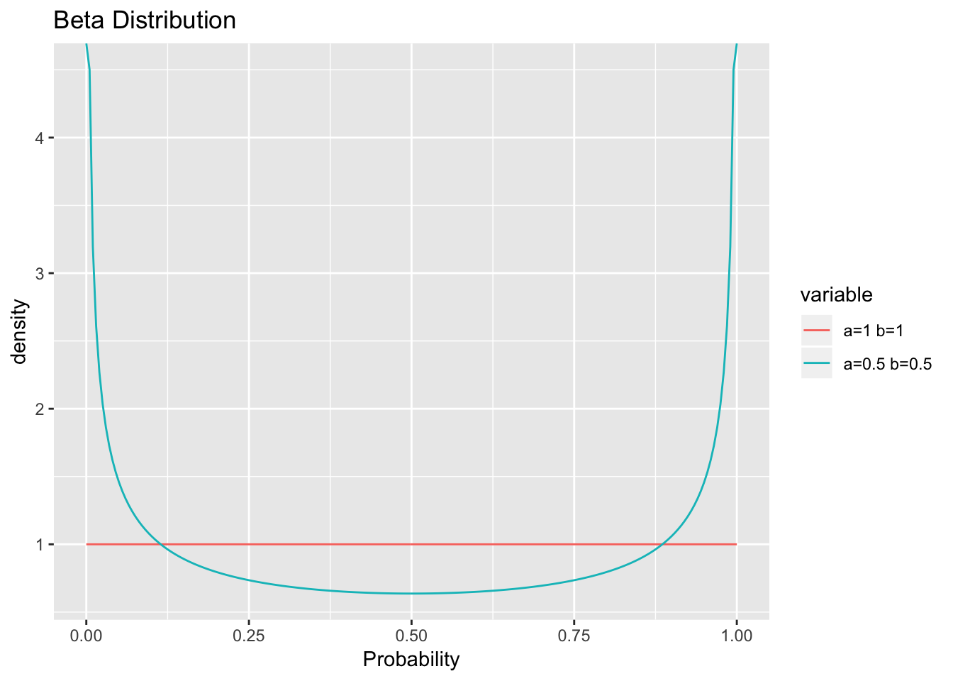

Here, we see that the Jeffreys prior compensates for the likelihood by weighting the extremes. Under the likelihood, data around $p=0.5$ has the least effect on the posterior, while data that shows a true $p=0$ or $p=1$ will have the greatest effect on the posterior. The Jeffreys prior is noninformative because it weights the opposite of the likelihood function while a flat prior would not. In this case, the Jeffreys prior happens to be a conjugate prior, though this is not always true.